Direct GPQR

import os

import torch
from torch.distributions import Normal
from gpytorch.variational import CholeskyVariationalDistribution
from gpytorch.variational import VariationalStrategy, LMCVariationalStrategy
from gpytorch.means import ConstantMean
from gpytorch.kernels import RBFKernel, ScaleKernel
from gpytorch.mlls import VariationalELBO
import matplotlib.pyplot as plt

from gpytorch_qr.models import DirectQuantileGP
from gpytorch_qr.likelihoods import (
    DirectQuantileLikelihood,
    MultiOutputDirectQuantileLikelihood,
)

try:
    import sys

    sys.path.insert(0, os.path.abspath(".."))

    import config_notebook
except ImportError:
    print("Output will not be deterministic SVG.")

torch.manual_seed(42)
device = torch.device("cuda" if torch.cuda.is_available() else "cpu")

n_epochs = int(os.getenv("GPYTORCHQR_N_EPOCHS", 5000))

Data preparation

def mean1(x):
    return torch.cos(x * 2 * 3.14)


def mean2(x):
    return torch.sin(x * 2 * 3.14)


def std(x):
    return x + 0.1


x_range = torch.linspace(0, 1, 100).reshape(-1, 1).to(device)
x = x_range.repeat(5, 1)
y1 = mean1(x) + torch.randn(x.shape, device=device).mul(std(x))
y2 = mean2(x) + torch.randn(x.shape, device=device).mul(std(x))
y = torch.concatenate([y1, y2], dim=-1)

q1 = torch.tensor([0.1, 0.5, 0.9], device=device)
true_quantiles1 = mean1(x_range) + Normal(0, std(x_range)).icdf(q1)

q2 = torch.tensor([0.1, 0.25, 0.5, 0.75, 0.9], device=device)
true_quantiles2 = mean2(x_range) + Normal(0, std(x_range)).icdf(q2)

x_pred = torch.linspace(0, 1.5, 100).reshape(-1, 1).to(device)

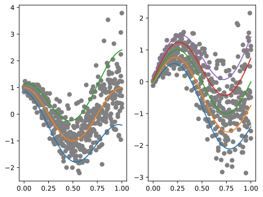
fig, axes = plt.subplots(1, 2)

axes[0].scatter(x.cpu(), y1.cpu(), c="gray")
axes[0].plot(x_range.cpu(), true_quantiles1.cpu())

axes[1].scatter(x.cpu(), y2.cpu(), c="gray")
axes[1].plot(x_range.cpu(), true_quantiles2.cpu())

fig.show()

Define model and likelihood

class MyGP(DirectQuantileGP):
    def __init__(self, inducing_points, num_quantiles, num_latents):
        N, D = inducing_points.size()
        variational_distribution = CholeskyVariationalDistribution(
            N,
            batch_shape=torch.Size([num_latents]),
        )
        variational_strategy = LMCVariationalStrategy(
            VariationalStrategy(
                self,
                inducing_points,
                variational_distribution,
                learn_inducing_locations=True,
            ),
            num_tasks=num_quantiles,
            num_latents=num_latents,
        )

        mean_module = ConstantMean(batch_shape=torch.Size([num_latents]))
        covar_module = ScaleKernel(
            RBFKernel(ard_num_dims=D, batch_shape=torch.Size([num_latents])),
            batch_shape=torch.Size([num_latents]),
        )
        super().__init__(variational_strategy, mean_module, covar_module)


inducing_points = torch.linspace(0, 1, 10).reshape(-1, 1).to(device)
num_latents = len(q1) + len(q2)
gp = MyGP(inducing_points, len(q1) + len(q2), num_latents=num_latents).to(device)
likelihood = MultiOutputDirectQuantileLikelihood(
    DirectQuantileLikelihood(q1),
    DirectQuantileLikelihood(q2),
).to(device)

Train

gp.train()
likelihood.train()
mll = VariationalELBO(likelihood, gp, num_data=len(y))
optimizer = torch.optim.Adam(
    list(gp.parameters()) + list(likelihood.parameters()),
    lr=0.001,
)

for _ in range(n_epochs):
    output = gp(x)
    loss = -mll(output, y)
    loss.backward()
    optimizer.step()
    optimizer.zero_grad()

gp.eval()
with torch.no_grad():
    mean_q = gp.mean_quantiles(x_pred)
    lower_q, upper_q = gp.quantile_quantiles(
        x_pred, torch.tensor([0.025, 0.975]).to(device)
    )

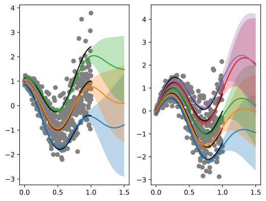
fig, axes = plt.subplots(1, 2)

axes[0].scatter(x.cpu(), y1.cpu(), c="gray")
axes[0].plot(x_range.cpu(), true_quantiles1.cpu(), color="k")
for i in range(len(q1)):
    axes[0].plot(x_pred.cpu(), mean_q[:, i].cpu(), label=f"q={q1[i].item():.2f}")
    axes[0].fill_between(
        x_pred.cpu().squeeze(),
        lower_q[:, i].cpu(),
        upper_q[:, i].cpu(),
        alpha=0.3,
    )

axes[1].scatter(x.cpu(), y2.cpu(), c="gray")
axes[1].plot(x_range.cpu(), true_quantiles2.cpu(), color="k")
for i in range(len(q2)):
    axes[1].plot(
        x_pred.cpu(), mean_q[:, len(q1) + i].cpu(), label=f"q={q2[i].item():.2f}"
    )
    axes[1].fill_between(
        x_pred.cpu().squeeze(),
        lower_q[:, len(q1) + i].cpu(),
        upper_q[:, len(q1) + i].cpu(),
        alpha=0.3,
    )

fig.show()