Module reference#
Gaussian process models#
Gaussian process classes for quantile regression.
- class gpytorch_qr.models.QuantileGP(variational_strategy, mean_module, covar_module)[source]#
Base class for Gaussian process quantile regression.
- Parameters:
- variational_strategygpytorch.variational.VariationalStrategy
- mean_modulegpytorch.means.Mean
- covar_modulegpytorch.kernels.Kernel
Notes
Input predictors are expected to have shape
(*B, N, D), where*Bare optional batch shapes (e.g., for cross validation), N is the number of data points and D is the number of input dimensions.Quantiles are task dimension with shape T, constructed by combination of L latent GPs.
variational_strategymust wrap a variational distribution with batch shape(*B, L).mean_moduleandcovar_modulemust have batch shape(*B, L).Posterior is
gpytorch.distributions.MultitaskMultivariateNormalwith batch shape(*B)and event shape(N, T).MLL loss is a tensor of shape
(*B).
- forward(x)[source]#
Define the computation performed at every call.
Should be overridden by all subclasses.
Note
Although the recipe for forward pass needs to be defined within this function, one should call the
Moduleinstance afterwards instead of this since the former takes care of running the registered hooks while the latter silently ignores them.
- abstractmethod joint_quantile_posterior(x)[source]#
Joint posterior over quantiles at input locations.
- Parameters:
- xtorch.Tensor with shape
(*B, N, D) The input locations.
- xtorch.Tensor with shape
- Returns:
- torch.distributions.Distribution
- marginal_quantile_posterior(x)[source]#
Marginal posterior over quantiles at input locations.
- Parameters:
- xtorch.Tensor with shape
(*B, N, D) The input locations.
- xtorch.Tensor with shape
- Returns:
- torch.distributions.Distribution
- mean_quantiles(x)[source]#
Predict quantiles by analytical posterior mean.
- Parameters:
- xtorch.Tensor with shape
(*B, N, D) The input locations.
- xtorch.Tensor with shape
- Returns:
- quantilestorch.Tensor
The predicted quantiles at the input locations.
- mean_quantiles_mc(x, num_samples=10)[source]#
Posterior mean of quantiles by Monte Carlo approximation.
- Parameters:
- xtorch.Tensor with shape
(*B, N, D) The input locations.
- num_samplesint, default=10
The number of Monte Carlo samples.
- xtorch.Tensor with shape
- Returns:
- quantilestorch.Tensor
The predicted quantiles at the input locations.
- mean_quantiles_delta(x)[source]#
Posterior mean of quantiles by 0th-order delta method.
- Parameters:
- xtorch.Tensor with shape
(*B, N, D) The input locations.
- xtorch.Tensor with shape
- Returns:
- quantilestorch.Tensor
The predicted quantiles at the input locations.
- quantile_quantiles(x, q)[source]#
Analytic quantile of quantile posterior.
- Parameters:
- xtorch.Tensor with shape
(*B, N, D) The input locations.
- qtorch.Tensor with shape (q,)
The quantile levels.
- xtorch.Tensor with shape
- Returns:
- quantilestorch.Tensor
The predicted quantiles at the input locations.
- quantile_quantiles_mc(x, q, num_samples=10)[source]#
Quantile of quantile posterior by Monte Carlo approximation.
- Parameters:
- xtorch.Tensor with shape
(*B, N, D) The input locations.
- qtorch.Tensor with shape (q,)
The quantile levels.
- num_samplesint, default=10
The number of Monte Carlo samples.
- xtorch.Tensor with shape
- Returns:
- quantilestorch.Tensor
The predicted quantiles at the input locations.
- class gpytorch_qr.models.DirectQuantileGP(variational_strategy, mean_module, covar_module)[source]#
Gaussian process quantile regression with direct quantile representation.
Notes
The task dimension of the output GP is structured as
[*Q_1, *Q_2, ..., *Q_k]
where
Q_icontains quantiles for the i-th output dimension.- joint_quantile_posterior(x)[source]#
Joint posterior over quantiles at input locations.
- Parameters:
- xtorch.Tensor with shape
(*B, N, D) The input locations.
- xtorch.Tensor with shape
- Returns:
- torch.distributions.Distribution
- marginal_quantile_posterior(x)[source]#
Marginal posterior over quantiles at input locations.
- Parameters:
- xtorch.Tensor with shape
(*B, N, D) The input locations.
- xtorch.Tensor with shape
- Returns:
- torch.distributions.Distribution
- mean_quantiles(x)[source]#
Predict quantiles by analytical posterior mean.
- Parameters:
- xtorch.Tensor with shape
(*B, N, D) The input locations.
- xtorch.Tensor with shape
- Returns:
- quantilestorch.Tensor
The predicted quantiles at the input locations.
- class gpytorch_qr.models.CenterGapQuantileGP(variational_strategy, mean_module, covar_module, num_quantiles, num_lower_quantiles)[source]#
Gaussian process quantile regression with center-gap quantile representation.
- Parameters:
- variational_strategy
- mean_modulegpytorch_qr.centergap.CenterGapMean
Mean module for center-gap representation.
- covar_module
- num_quantileslist of int
The number of quantiles in each output dimension.
- num_lower_quantileslist of int
The number of lower quantiles in each output dimension for center-gap representation.
Notes
The task dimension of the output GP is structured as
[c_1, c_2, ..., c_k, *L_1, *U_1, *L_2, *U_2, ..., *L_k, *U_k]
where
c_iis the central quantile for the i-th output dimension,L_icontains the pre-softplus-transformed lower gaps, andU_icontains the pre-softplus-transformed upper gaps.
Asymmetric laplace distribution#
Asymmetric Laplace distributions for Bayesian quantile regression.
- class gpytorch_qr.distributions.ALD(m, lamda, kappa)[source]#
Asymmetric Laplace distribution.
- Parameters:
- mtorch.Tensor
The location parameter of the distribution.
- lamdatorch.Tensor
The scale parameter of the distribution.
- kappatorch.Tensor
The asymmetry parameter of the distribution.
- Attributes:
- mtorch.Tensor
- lamdatorch.Tensor
- kappatorch.Tensor
- class gpytorch_qr.distributions.QuantileALD(m, lamda, kappa)[source]#
Asymmetric Laplace distribution for multiple quantiles.
- Parameters:
- mtorch.Tensor with shape
(S, *B, N, Q) The location parameters of the distribution.
- lamdatorch.Tensor with shape
(*B, 1, Q) The scale parameters of the distribution for each quantile.
- kappatorch.Tensor with shape
(*B, 1, Q) The quantile levels of the distribution.
- mtorch.Tensor with shape
- Attributes:
- mtorch.Tensor with shape
(S, *B, N, Q) - lamdatorch.Tensor with shape
(1, *B, 1, Q) - kappatorch.Tensor with shape
(1, *B, 1, Q)
- mtorch.Tensor with shape
Notes
This class is designed for univariate Bayesian quantile regression with multiple quantiles, i.e.,
yis a vector of univariate response from which multiple quantiles are estimated.S: the number of samples drawn from the posterior distribution.Q: the number of quantiles.B: additional batches.N: the number of data points.
Although the response is univariate, the distribution is multitask where each task corresponds to a different quantile. Multivariate regression with multiple quantiles can be achieved by defining a likelihood class that uses multiple instances of this distribution.
- log_prob(value)[source]#
Log probability of the asymmetric Laplace distribution at the given value.
- Parameters:
- valuetorch.Tensor with shape
(*B, N, 1)or(*B, N, Q) Observed response variables at which to evaluate the log probability.
- valuetorch.Tensor with shape
- Returns:
- logptorch.Tensor with shape
(S, *B, N, Q) The log probability at the given values for each task and sample.
- logptorch.Tensor with shape
Asymmetric laplace likelihood#
Asymmetric Laplace distributions likelihoods for quantile regression.
- class gpytorch_qr.likelihoods.DirectQuantileLikelihood(kappa, raw_scales=0.0, learn_scales=True)[source]#
Likelihood for single-output multi-quantile GPQR with direct representation.
- Parameters:
- kappatorch.Tensor with shape
(*B, Q) The quantile levels.
- raw_scalestorch.Tensor with shape
(*B, Q)or scalar, default=0 The initial untransformed scales of the asymmetric Laplace distribution.
- learn_scales
- kappatorch.Tensor with shape
- Attributes:
- kappatorch.Tensor with shape
(*B, Q) - raw_scalestorch.Tensor with shape
(*B, Q)
- kappatorch.Tensor with shape
Notes
The task dimension of the input GP posterior should be structured as
[q_1, q_2, ..., q_Q]
where
q_iis the i-th quantile function.- forward(function_samples)[source]#
Return the ALD distribution for the given function samples.
- Parameters:
- function_samplestorch.Tensor with shape
(S, *B, N, Q) The function samples drawn from the GP posterior distribution. S is the number of samples, Q is the number of tasks, B is the batch shape, and N is the number of data points.
- function_samplestorch.Tensor with shape
- Returns:
- QuantileALD
- class gpytorch_qr.likelihoods.CenterGapQuantileLikelihood(kappa, central_quantile_index, raw_scales=0.0, learn_scales=True)[source]#
Likelihood for single-output multi-quantile GPQR with center-gap representation.
- Parameters:
- kappatorch.Tensor with shape
(*B, Q) The quantile levels.
- central_quantile_indexint
The index of the central quantile in the quantile levels.
- raw_scalestorch.Tensor with shape
(*B, Q)or scalar, default=0 The initial untransformed scales of the asymmetric Laplace distribution.
- learn_scales
- kappatorch.Tensor with shape
- Attributes:
- kappatorch.Tensor with shape
(*B, Q) - raw_scalestorch.Tensor with shape
(*B, Q)
- kappatorch.Tensor with shape
Notes
The task dimension of the input GP posterior should be structured as
[c, *L, *U]
where
cis the central quantile,Lcontains the pre-softplus-transformed lower gaps, andUcontains the pre-softplus-transformed upper gaps.Examples
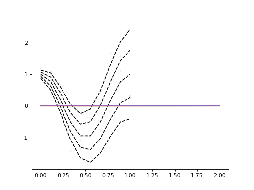
>>> import torch
>>> from torch.distributions import Normal
>>> torch.manual_seed(42)
>>> def mean(x):
...     return torch.cos(x * 2 * 3.14)
>>> def std(x):
...     return x + 0.1
>>> x_range = torch.linspace(0, 1, 10).reshape(-1, 1)
>>> x = x_range.repeat(2, 1)
>>> y = (mean(x) + torch.randn(x.shape).mul(std(x))).squeeze()
>>> q = torch.tensor([0.1, 0.25, 0.5, 0.75, 0.9])
>>> true_quantiles = mean(x_range) + std(x_range) * Normal(0, 1).icdf(q)
>>> from gpytorch.variational import CholeskyVariationalDistribution
>>> from gpytorch.variational import VariationalStrategy
>>> from gpytorch.means import ConstantMean
>>> from gpytorch.kernels import RBFKernel, ScaleKernel
>>> from gpytorch_qr.means import CenterGapMean
>>> from gpytorch_qr.models import CenterGapQuantileGP
>>> from gpytorch_qr.likelihoods import CenterGapQuantileLikelihood
>>> from gpytorch_qr.variational import CenterGapLMCVariationalStrategy
>>> class MyGP(CenterGapQuantileGP):
...     def __init__(
...         self,
...         inducing_points,
...         num_q,
...         num_lower_q,
...         num_latents,
...     ):
...         N, D = inducing_points.size()
...         variational_distribution = CholeskyVariationalDistribution(
...             N,
...             batch_shape=torch.Size([num_latents]),
...         )
...         var_strat = CenterGapLMCVariationalStrategy(
...             VariationalStrategy(
...                 self,
...                 inducing_points,
...                 variational_distribution,
...                 learn_inducing_locations=True,
...             ),
...             num_q,
...             num_latents,
...             num_quantiles=[num_q],
...             num_lower_quantiles=[num_lower_q],
...         )
...         mean = CenterGapMean(
...             ConstantMean(batch_shape=torch.Size([1])),
...             ConstantMean(batch_shape=torch.Size([num_latents - 1])),
...         )
...         covar = ScaleKernel(
...             RBFKernel(ard_num_dims=D, batch_shape=torch.Size([num_latents])),
...             batch_shape=torch.Size([num_latents]),
...         )
...         super().__init__(var_strat, mean, covar, [num_q], [num_lower_q])
>>> inducing_pts = torch.linspace(0, 1, 10).reshape(-1, 1)
>>> central_q_index = (q - 0.5).abs().argmin().item()
>>> num_latents = len(q) - 2  # recommended to be smaller than q
>>> gp = MyGP(inducing_pts, len(q), central_q_index, num_latents)
>>> likelihood = CenterGapQuantileLikelihood(q, central_q_index)
>>> from gpytorch.mlls import VariationalELBO
>>> gp.train()
>>> likelihood.train()
>>> mll = VariationalELBO(likelihood, gp, num_data=y.numel())
>>> optimizer = torch.optim.Adam(
...     list(gp.parameters()) + list(likelihood.parameters()),
...     lr=0.001,
... )
>>> N = 1  # Set to 1 for faster training; increase for better performance
>>> for _ in range(N):
...     output = gp(x)
...     loss = -mll(output, y)
...     loss.backward()
...     optimizer.step()
...     optimizer.zero_grad()
>>> gp.eval()
>>> x_pred = torch.linspace(0, 2, 100).reshape(-1, 1)
>>> with torch.no_grad():
...     quantiles = gp.mean_quantiles_mc(x_pred)
>>> import matplotlib.pyplot as plt
>>> plt.scatter(x, y, c='gray', marker='.', alpha=0.1)
>>> plt.plot(x_range, true_quantiles, '--', c='k')
>>> plt.plot(x_pred, quantiles)
- forward(function_samples)[source]#
Return the ALD distribution for the given function samples.
- Parameters:
- function_samplestorch.Tensor with shape
(S, *B, N, Q) The function samples drawn from the GP posterior distribution. S is the number of samples, Q is the number of tasks, B is the batch shape, and N is the number of data points.
- function_samplestorch.Tensor with shape
- Returns:
- QuantileALD
- class gpytorch_qr.likelihoods.MultiOutputDirectQuantileLikelihood(*likelihoods)[source]#
Likelihood for multi-output multi-quantile direct GPQR.
- Parameters:
- *likelihoodslist of DirectQuantileLikelihood
Notes
The task dimension of the input GP posterior should be structured as
[*Q_1, *Q_2, ..., *Q_k]
where
Q_icontains quantiles for the i-th output dimension.- forward(function_samples)[source]#
Return the ALD distribution for the given function samples.
- Parameters:
- function_samplestorch.Tensor with shape
(S, *B, N, Q) The function samples drawn from the GP posterior distribution. S is the number of samples, Q is the number of tasks, B is the batch shape, and N is the number of data points.
- function_samplestorch.Tensor with shape
- Returns:
- QuantileALD
- class gpytorch_qr.likelihoods.MultiOutputCenterGapQuantileLikelihood(*likelihoods)[source]#
Likelihood for multi-output multi-quantile center-gap GPQR.
- Parameters:
- *likelihoodslist of CenterGapQuantileLikelihood
Notes
The task dimension of the input GP posterior should be structured as
[c_1, c_2, ..., c_k, *L_1, *U_1, *L_2, *U_2, ..., *L_k, *U_k]
where
c_iis the central quantile for the i-th output dimension,L_icontains the pre-softplus-transformed lower gaps, andU_icontains the pre-softplus-transformed upper gaps.- forward(function_samples)[source]#
Return the ALD distribution for the given function samples.
- Parameters:
- function_samplestorch.Tensor with shape
(S, *B, N, Q) The function samples drawn from the GP posterior distribution. S is the number of samples, Q is the number of tasks, B is the batch shape, and N is the number of data points.
- function_samplestorch.Tensor with shape
- Returns:
- QuantileALD
Variational strategies#
Variational strategies for GPQR.
- class gpytorch_qr.variational.CenterGapLMCVariationalStrategy(base_variational_strategy, num_tasks, num_latents, latent_dim=-1, jitter_val=None, num_quantiles=None, num_lower_quantiles=None)[source]#
Special LMC variational strategy for the center-gap representation.
This class forces the following structure:
Each central quantile of each output dimension is directly represented by a dedicated independent latent function.
Gap functions for all output dimensions are represented by linear combinations of the remaining latent functions.
Only the coefficients for the gap functions are learned.
- Parameters:
- base_variational_strategy
- num_tasks
- num_latents
- latent_dim
- jitter_val
- num_quantileslist of int, optional
The number of quantiles in each output dimension. Its sum must equal num_tasks. If not passed, defaults to
[num_tasks], i.e., output is assumed to be 1-dimensional.- num_lower_quantileslist of int, optional
The number of lower quantiles in each output dimension for center-gap representation. If not passed, defaults to a balanced split of the quantiles.
See also
gpytorch_qr.means.CenterGapMeanMean module for this strategy to place prior mean on latent functions.
Notes
This class is introduced to facilitate implementing center-gap model where the gaps are correlated while the center has prior mean.
The first
klatent functions directly represent the central quantiles of each output dimension, and they do not form any linear combinations with the other latent functions. The remaining latent functions are linearly combined to model the gap functions between quantiles.The input
Tlatent GPs are structured as[c_1, c_2, ..., c_k, g_1, g_2, ..., g_{T-k}]where:
c_iis the central quantile for i-th output dimension,g_jis the j-th latent function for modeling the gaps between quantiles.
The output multitask GPs are structured as
[c_1, c_2, ..., c_k, *L_1, *U_1, *L_2, *U_2, ..., *L_k, *U_k]
where:
c_iis the central quantile for i-th output dimension,L_icontains pre-softplus-transformed lower gaps for i-th output dimension,U_icontains pre-softplus-transformed upper gaps for i-th output dimension.
Hint
The limitation of this class is that
It cannot correlate the central quantile and the gap functions.
It cannot correlate the central quantiles of different output dimensions.
Should such correlations be desired, one can modify the input observations by \(y \leftarrow y - \mu(x)\) and use a standard LMC variational strategy to model the residuals.
- classmethod construct_lmc_mask(T, Q, k)[source]#
Construct a mask to restrict the learnable LMC coefficients.
- Parameters:
- Tint
The number of latent functions.
- Qint
The number of quantiles.
- kint
The number of output dimensions.
- Returns:
- lmc_masktorch.Tensor with shape
(T, Q) A binary mask of the same shape as the LMC coefficients. 1 indicates learnable coefficients, and 0 indicates fixed coefficients.
- lmc_masktorch.Tensor with shape
Mean modules#
Mean modules.
- class gpytorch_qr.means.CenterGapMean(center_mean, gap_mean)[source]#
Mean module for the center-gap representation.
- Parameters:
- center_meangpytorch.means.Mean or torch.nn.ModuleList of gpytorch.means.Mean
Mean module for the central quantile. If a
torch.nn.ModuleListis provided, each of the contained mean modules applies to a different output dimension. Each mean should have batch shape(*B, 1).- gap_meangpytorch.means.Mean
Mean module for the quantile gaps. Should have batch shape
(*B, L-k)where L is the number of latent GPs and k is the number of output dimensions.
See also
gpytorch_qr.variational.CenterGapLMCVariationalStrategyLMC variational strategy that needs this mean module.
Notes
Input predictors are expected to have shape
(*B, 1, N, D). N is the number of data points and D is the number of input dimensions.Hint
If this mean is used with LMC variational strategy, the prior means will be placed on latent GPs instead of the output GPs. This may lead to unexpected behavior by the linear combination of the latent GPs.
Using
gpytorch_qr.variational.CenterGapLMCVariationalStrategyis a quick way to separate the prior means for the central quantiles and the gap functions.For more fundamental solution, consider modifying the input observations by \(y \leftarrow y - \mu(x)\) and use a standard LMC variational strategy to model the residuals.
Utilities#
Utility functions.
- gpytorch_qr.utils.centergap_to_quantiles(central, lower_gaps, upper_gaps)[source]#
Convert center-gap representation samples to quantiles.
- Parameters:
- centraltorch.Tensor with shape (…, 1)
The central quantile values.
- lower_gapstorch.Tensor with shape (…, L)
Pre-softplus-transformed lower gap values.
- upper_gapstorch.Tensor with shape (…, U)
Pre-softplus-transformed upper gap values.
- Returns:
- quantilestorch.Tensor with shape (…, Q)
Quantile values. (Q = L + U + 1) The quantiles are ordered in increasing order along the quantile dimension.
- class gpytorch_qr.utils.CenterGapToQuantileTransform(Qs, Ls)[source]#
Transformation from center-gap distribution to quantile distribution.
- Parameters:
- Qslist of int
The number of quantiles for each task, i.e.,
[Q_1, Q_2, ..., Q_k].- Lslist of int
The number of lower quantiles in center-gap representation for each task, i.e.,
[L_1, L_2, ..., L_k].
Notes
The input distribution’s quantile dimension should be laid out as:
[c_1, c_2, ..., c_k, *L_1, *U_1, *L_2, *U_2, ..., *L_k, *U_k]
where:
c_iis the central quantile for i-th output dimension,L_icontains pre-softplus-transformed lower gaps for i-th output dimension,U_icontains pre-softplus-transformed upper gaps for i-th output dimension.
The output distribution’s quantile dimension is laid out as:
[*Q_1, *Q_2, ..., *Q_k].
- gpytorch_qr.utils.transform_centergap_posterior(posterior, Qs, Ls)[source]#
Convert the center-gap posterior to quantile posterior.
- Parameters:
- posteriorgpytorch.distributions.MultitaskMultivariateNormal
The center-gap posterior distribution. Event shape must be
(N, Q_1 + Q_2 + ..., Q_k), whereQ_iis the number of quantiles for i-th output dimension.- Qslist of int
The number of quantiles for each task, i.e.,
[Q_1, Q_2, ..., Q_k].- Lslist of int
The number of lower quantiles in center-gap representation for each task, i.e.,
[L_1, L_2, ..., L_k].
- Returns:
- quantile_posteriortorch.distributions.TransformedDistribution
Posterior over quantiles, obtained by applying
CenterGapToQuantileTransformto a batchedgpytorch.distributions.MultitaskMultivariateNormal.
Notes
Input and output distribution has specific structure in the quantile dimension. See
CenterGapToQuantileTransformfor details.