GPQR Tutoral

Gaussian process quantile regression (GPQR) estimates quantile function using Gaussian process regression with asymmetric laplace distribution (ALD) likelihood.

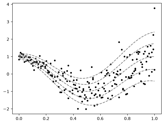
In this tutorial, we estimate multiple quantile levels using multitask learning for the following data with heteroscedastic noise:

\[Y = \cos(2\pi X) + \epsilon, \quad \epsilon \sim \mathcal{N}(0, X + 0.1).\]

To avoid quantile crossing, center-gap representation is used. Informative prior is applied by subtracting the prior mean from the observed \(Y\). Correlation between gaps are modeled by using linear model of coregionalization (LMC) of latent functions.

import os
import torch
import matplotlib.pyplot as plt

torch.manual_seed(42)
device = torch.device("cuda" if torch.cuda.is_available() else "cpu")

n_epochs = int(os.getenv("GPYTORCHQR_N_EPOCHS", 2500))

Input data

We generate sinusiodal data with heteroscedastic noise.

def mean(x):
    # x: (N, 1)
    return torch.cos(x.squeeze(-1) * 2 * 3.14)


def std(x):
    # x: (N, 1)
    return x.squeeze(-1) + 0.1


x_range = torch.linspace(0, 1, 100, device=device).reshape(-1, 1)
x = x_range.repeat(2, 1)
y = mean(x) + torch.randn(len(x), device=device).mul(std(x))
q = torch.tensor([0.1, 0.25, 0.5, 0.75, 0.9], device=device)
standard_normal = torch.distributions.Normal(
    torch.zeros((), device=device), torch.ones((), device=device)
)
icdf = standard_normal.icdf(q)
true_quantiles = mean(x_range).unsqueeze(1) + std(x_range).unsqueeze(1) * icdf

x_pred = torch.linspace(0, 1.5, 100, device=device).reshape(-1, 1)

plt.scatter(x.cpu(), y.cpu(), c="k", marker=".")
plt.plot(x_range.cpu(), true_quantiles.cpu(), "--", c="gray")
plt.show()

Prior mean

For simplicity, we place a non-learnable prior mean.

from gpytorch.means import Mean


class PriorMean(Mean):
    def forward(self, x):
        return mean(x)


prior_mean = PriorMean().to(device)

plt.scatter(x.cpu(), y.cpu(), c="k", marker=".")
plt.plot(x_pred.cpu(), prior_mean(x_pred).detach().cpu(), c="r")
plt.show()

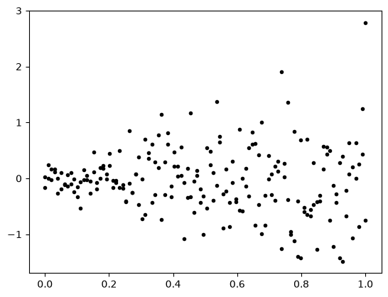
Then, the goal of Gaussian process regression becomes modeling the distribution of residual.

res = y - prior_mean(x)

plt.scatter(x.cpu(), res.cpu(), c="k", marker=".")
plt.show()

Gaussian process regression

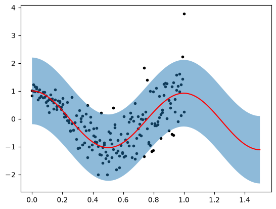
The standard GPR predicts the distribution of \(y\) to be homoscedastic.

from gpytorch.models import ExactGP
from gpytorch.means import ConstantMean
from gpytorch.kernels import ScaleKernel, RBFKernel
from gpytorch.distributions import MultivariateNormal
from gpytorch.likelihoods import GaussianLikelihood


class ExactGPModel(ExactGP):
    def __init__(self, train_x, train_y, likelihood):
        super(ExactGPModel, self).__init__(train_x, train_y, likelihood)
        self.mean_module = ConstantMean()
        self.covar_module = ScaleKernel(RBFKernel())

    def forward(self, x):
        mean_x = self.mean_module(x)
        covar_x = self.covar_module(x)
        return MultivariateNormal(mean_x, covar_x)


prior_mean = PriorMean().to(device)
likelihood = GaussianLikelihood().to(device)
model = ExactGPModel(x, res, likelihood).to(device)

from gpytorch.mlls import ExactMarginalLogLikelihood

model.train()
likelihood.train()
prior_mean.train()

optimizer = torch.optim.Adam(
    list(model.parameters()) + list(prior_mean.parameters()),
    lr=0.001,
)
mll = ExactMarginalLogLikelihood(likelihood, model)

for i in range(n_epochs):
    optimizer.zero_grad()

    output = model(x)
    loss = -mll(output, res)
    loss.backward()
    optimizer.step()

model.eval()
likelihood.eval()
prior_mean.eval()

with torch.no_grad():
    prior = prior_mean(x_pred)
    res_posterior = model(x_pred)
    res_predictive_posterior = likelihood(model(x_pred))

res_posterior_mean = res_posterior.mean
res_posterior_lower, res_posterior_upper = res_posterior.confidence_region()

posterior_mean = (prior + res_posterior_mean).detach().cpu()
posterior_lower = (prior + res_posterior_lower).detach().cpu()
posterior_upper = (prior + res_posterior_upper).detach().cpu()

plt.scatter(x.cpu(), y.cpu(), c="k", marker=".")
plt.plot(x_pred.cpu(), posterior_mean.detach().cpu(), c="r")
plt.fill_between(x_pred.cpu().squeeze(), posterior_lower, posterior_upper, alpha=0.5)
plt.show()

res_predictive_posterior_mean = res_predictive_posterior.mean
res_predictive_posterior_lower, res_predictive_posterior_upper = (
    res_predictive_posterior.confidence_region()
)

predictive_posterior_mean = (prior + res_predictive_posterior.mean).detach().cpu()
predictive_posterior_lower = (prior + res_predictive_posterior_lower).detach().cpu()
predictive_posterior_upper = (prior + res_predictive_posterior_upper).detach().cpu()

plt.scatter(x.cpu(), y.cpu(), c="k", marker=".")
plt.plot(x_pred.cpu(), predictive_posterior_mean, c="r")
plt.fill_between(
    x_pred.cpu().squeeze(),
    predictive_posterior_lower,
    predictive_posterior_upper,
    alpha=0.5,
)
plt.show()

Gaussian process quantile regression

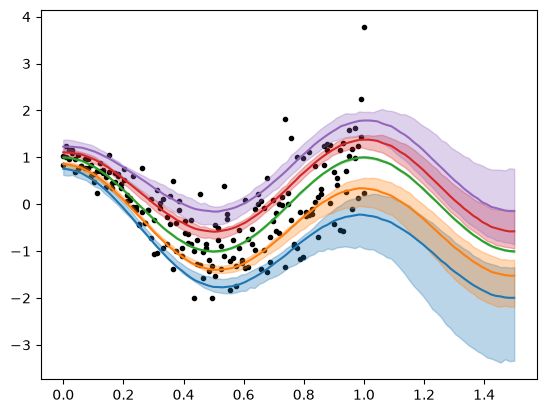
The GPQR learns the heteroscedastic distribution by modeling multiple quantile levels as latent functions.

from gpytorch.variational import (
    CholeskyVariationalDistribution,
    VariationalStrategy,
)
from gpytorch_qr.models import CenterGapQuantileGP
from gpytorch_qr.likelihoods import CenterGapQuantilesLikelihood
from gpytorch_qr.variational import CenterGapLMCVariationalStrategy


class QuantileGPModel(CenterGapQuantileGP):
    def __init__(
        self,
        inducing_points,
        num_quantiles,
        num_lower_quantiles,
        num_latents,
    ):
        N, D = inducing_points.size()
        variational_distribution = CholeskyVariationalDistribution(
            N,
            batch_shape=torch.Size([num_latents]),
        )
        variational_strategy = CenterGapLMCVariationalStrategy(
            VariationalStrategy(
                self,
                inducing_points,
                variational_distribution,
                learn_inducing_locations=True,
            ),
            num_quantiles,
            num_latents,
        )

        mean = ConstantMean(batch_shape=torch.Size([num_latents]))
        covar = ScaleKernel(
            RBFKernel(ard_num_dims=D, batch_shape=torch.Size([num_latents])),
            batch_shape=torch.Size([num_latents]),
        )
        super().__init__(
            variational_strategy, mean, covar, [num_quantiles], [num_lower_quantiles]
        )


inducing_points = torch.linspace(0, 1, 10, device=device).reshape(-1, 1)
central_q_index = 2
num_latents = 3

prior_mean = PriorMean().to(device)
likelihood = CenterGapQuantilesLikelihood(q, central_q_index).to(device)
model = QuantileGPModel(
    inducing_points,
    len(q),
    central_q_index,
    num_latents,
).to(device)

from gpytorch.mlls import VariationalELBO

model.train()
likelihood.train()
prior_mean.train()

optimizer = torch.optim.Adam(
    list(model.parameters()) + list(likelihood.parameters()),
    lr=0.001,
)
mll = VariationalELBO(likelihood, model, num_data=y.numel())

for _ in range(n_epochs):
    output = model(x)
    loss = -mll(output, res)
    loss.backward()
    optimizer.step()
    optimizer.zero_grad()

model.eval()
likelihood.eval()
prior_mean.eval()

with torch.no_grad():
    pred_prior_mean = prior_mean(x_pred).unsqueeze(-1)
    mean_q = model.mean_quantiles_mc(x_pred)
    lower_q, upper_q = model.quantile_quantiles_mc(
        x_pred, torch.tensor([0.025, 0.975], device=device)
    )

pred_mean_q = (pred_prior_mean + mean_q).detach().cpu()
pred_lower_q = (pred_prior_mean + lower_q).detach().cpu()
pred_upper_q = (pred_prior_mean + upper_q).detach().cpu()

colors = plt.cm.tab10.colors

plt.scatter(x.cpu(), y.cpu(), c="k", marker=".")

for i in range(len(q)):
    plt.plot(x_pred.cpu(), pred_mean_q[:, i].cpu(), color=colors[i])
    plt.fill_between(
        x_pred.cpu().squeeze(),
        pred_lower_q[:, i].cpu(),
        pred_upper_q[:, i].cpu(),
        color=colors[i],
        alpha=0.3,
    )
plt.show()